Getting started with evofr
We begin by loading pandas to process our data from a .tsv file to a pandas.DataFrame. We also load evofr which will be used to specify our data format for pre-processing, the model we’ll used for estimation, and our inference method.
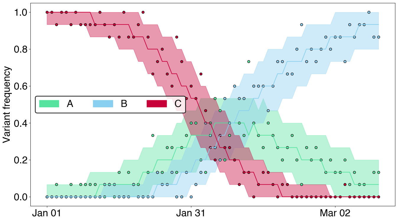
In what follows, we use the ef.VariantFrequencies dataspec which will handle formatting the data for input to our model.
[1]:
import pandas as pd
import evofr as ef
[2]:
# Getting data
raw_seq = pd.read_csv("../../test/testing_data/mlr-variant-counts.tsv", sep="\t")
raw_seq = raw_seq[raw_seq.location == "City0"]
variant_frequencies = ef.VariantFrequencies(raw_seq, pivot="C")
In evofr, we can specify a model by just calling a model constructor. The simplest model in evofrfor relative fitness estimation which takes in the generation time which we’ll use to convert from relative fitness to growth advantage.
Underneath the hood, this model is estimating initial variant frequencies \(f_v(0)\) and relative fitness \(\lambda_v\), so that our variant frequencies over time \(f_v(t)\) can be written as
where we fix \(\alpha_{u^*} = \beta_{u^*} = 0\) for some pivot variant u^*. This idea of a pivot variant is maintained with these frequency-based models can be specified withe pivot arugment in the ef.VariantFrequencies constructor.
[3]:
# Defining model
mlr = ef.MultinomialLogisticRegression(tau=4.2)
In this example, we’ll use Markov Chain Monte Carlo (MCMC) sampling via the NUTS sampler for 1000 warmup samples and 1000 samples.
[4]:
# Defining inference method
inference_method = ef.InferNUTS(num_samples=1000, num_warmup=1000)
From here, getting our posterior and running our model is as simple as running the following line of code.
[5]:
# Fitting model
posterior = inference_method.fit(mlr, variant_frequencies)
sample: 100%|█████████████████████████████████████████| 2000/2000 [00:00<00:00, 2316.21it/s, 15 steps of size 1.01e-01. acc. prob=0.95]
This ef.PosteriorHandler object will contain our data (attribute: data) and estimated parameters (attribute: samples).
[6]:
# Forecasting using the model and posterior samples
forecast_L = 50
posterior.samples = mlr.forecast_frequencies(posterior.samples, forecast_L)
Handling model results
We can save and load posteriors using commands on the posterior such as posterior.save_posterior and posterior.load_posterior. The current supported outputs are json and pickle.
[7]:
posterior.save_posterior("mlr_estimates.pkl")
# Loading new posterior
loaded_posterior = ef.PosteriorHandler(data=variant_frequencies).load_posterior("mlr_estimates.pkl")
Exporting as DataFrames
[8]:
# TODO:
Plotting model results
There are several methods and classes implementing for taking a quick glance at your data.
[9]:
import matplotlib
import matplotlib.pyplot as plt
import matplotlib.transforms as mtransforms

font = {'family' : 'Helvetica',
        'weight' : 'light',
        'size'   : 24}

matplotlib.rc('font', **font)
[10]:
ps = [0.95, 0.8, 0.5]
alphas = [0.2, 0.4, 0.6]


v_colors = ["#56e39f", "#89CFF0", "#C70039"]
v_names = ['A', 'B', 'C']
color_map = {v : c for c, v in zip(v_colors, v_names)}
[11]:
from evofr.plotting import FrequencyPlot, GrowthAdvantagePlot, PatchLegend, add_dates_sep
from evofr.plotting import plot_site_in_time, plot_variants, plot_time_series_with_variants
[12]:
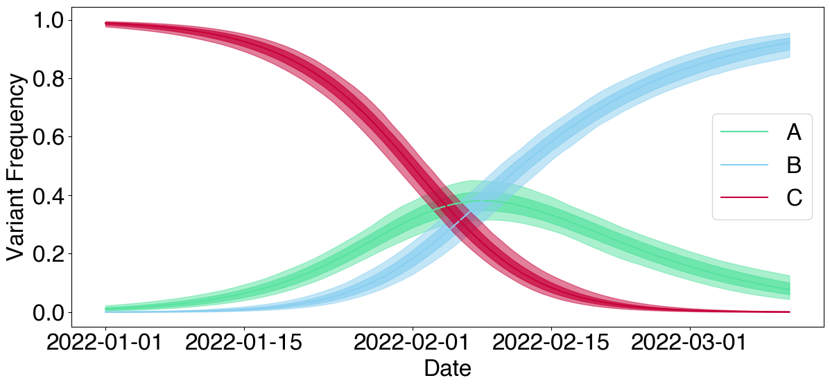
# Plot predicted frequencies
fig = plt.figure(figsize=(14, 8))
gs = fig.add_gridspec(nrows=1, ncols=1)
ax = fig.add_subplot(gs[0,0])

FrequencyPlot(posterior, color_map=color_map).plot(ax, forecast=True)
ax.axvline(x=len(variant_frequencies.dates)-1, color='k', linestyle='--') # Adding forecast cut off
add_dates_sep(ax, ef.data.expand_dates(variant_frequencies.dates, forecast_L), sep=30) # Adding dates
PatchLegend(color_map).add_legend(ax)

fig.tight_layout()
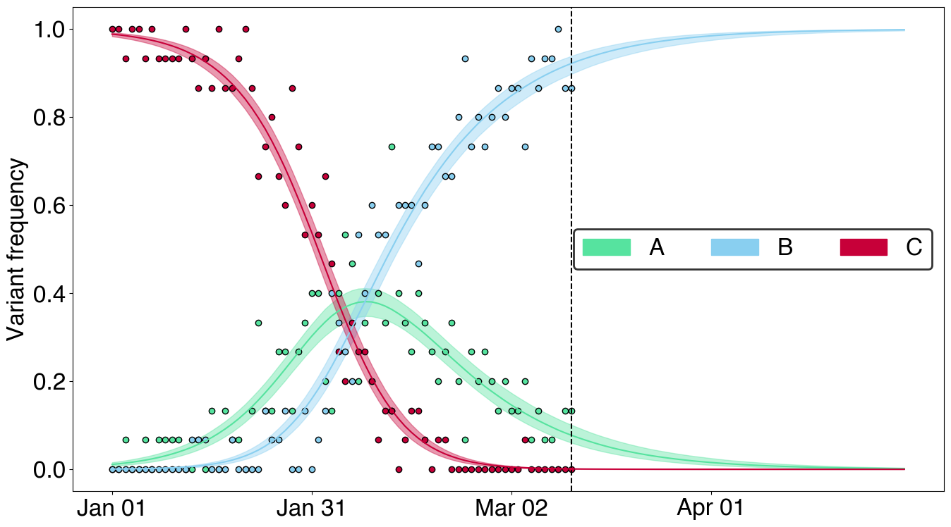
[13]:
# Plot posterior predictive frequency
fig = plt.figure(figsize=(14, 8))
gs = fig.add_gridspec(nrows=1, ncols=1)
ax = fig.add_subplot(gs[0,0])

FrequencyPlot(posterior, color_map=color_map).plot(ax, posterior=False, predictive=True)
add_dates_sep(ax, variant_frequencies.dates, sep=30) # Adding dates
PatchLegend(color_map).add_legend(ax)
fig.tight_layout()
[14]:
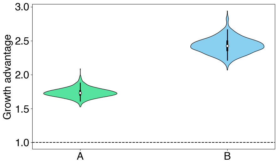
# Plotting growth advantage
fig = plt.figure(figsize=(10, 6))
gs = fig.add_gridspec(nrows=1, ncols=1)
ax = fig.add_subplot(gs[0,0])

GrowthAdvantagePlot(posterior, color_map=color_map).plot(ax=ax)
[14]:
<evofr.plotting.plotting_classes.GrowthAdvantagePlot at 0x316280590>
[15]:
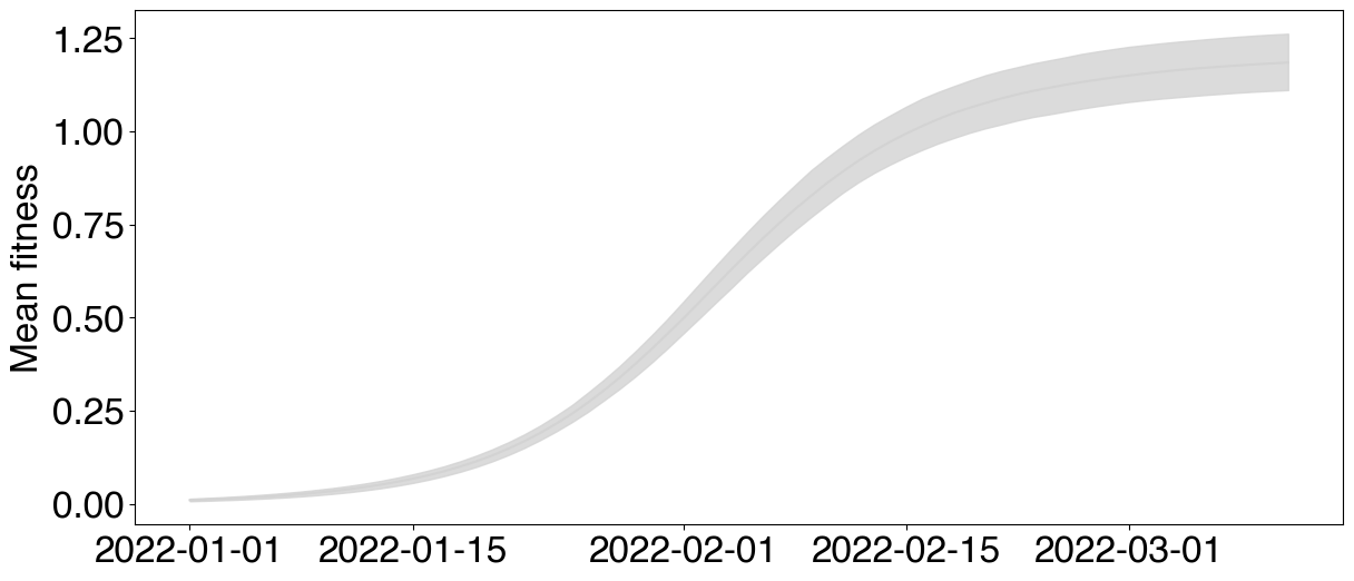
# Computing and plotting mean fitness using `plot_site_in_time` primitive
fig, ax = plt.subplots(figsize=(14,6))
posterior.samples["delta_bar"] = (posterior.samples["freq"][:, :, :-1] * posterior.samples["ga"][:, None, :]).mean(axis=-1)
plot_site_in_time(ax, posterior.samples, "delta_bar", dates = posterior.data.dates, alphas=[0.8], colors="lightgray", quantiles=[0.8])
ax.set_ylabel("Mean fitness")
[15]:
Text(0, 0.5, 'Mean fitness')
[16]:
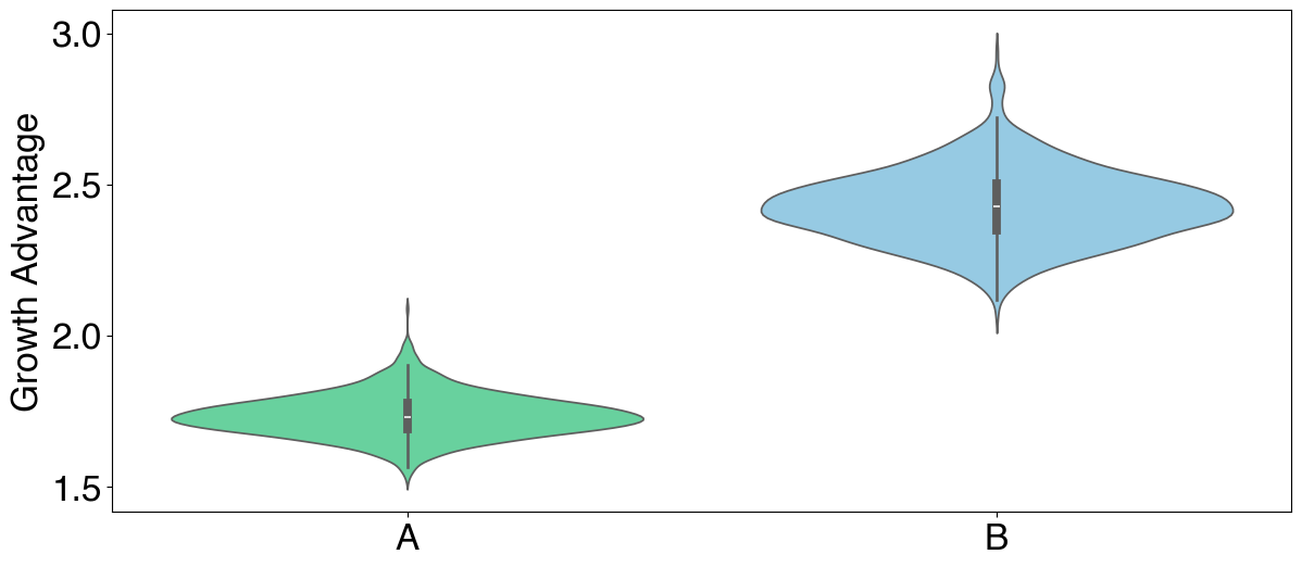
# Plotting growth advantage using `plot_variants` primitive
fig, ax = plt.subplots(figsize=(14,6))
plot_variants(ax,
              posterior.samples,
              "ga",
              color_map=color_map,
              variants=posterior.data.var_names,
              variants_to_plot = ["A", "B"])
ax.set_ylabel("Growth Advantage")
[16]:
Text(0, 0.5, 'Growth Advantage')
[17]:
# Plotting variant frequency using `plot_time_series_with_variants` primitive
fig, ax = plt.subplots(figsize=(14,6))
plot_time_series_with_variants(ax,
                               posterior.samples, "freq",
                               variants=posterior.data.var_names,
                               dates = posterior.data.dates,
                               color_map=color_map,
                               alphas = [0.5, 0.7],
                               quantiles=[0.99, 0.8]
)
ax.set_ylabel("Variant Frequency")
[17]:
Text(0, 0.5, 'Variant Frequency')